What can Bass’ mathematical approach to innovation diffusion tell/show us? Well, quite a lot. We can:

• explore the impact of innovators (those in the social system that are external influences) and imitators (those internally influenced)
• predict the diffusion of our innovation – allowing us to understand when to ramp up service provision capability (or product supply lines)
• get a more accurate sizing of adopter types (so we can distribute our marketing budgets better)
• understand the best timing to launch the next generation of an innovation
• evaluate the market value of a business

Exciting stuff, right? Even more impressively, we get to explore the model hands-on in Excel.

(You can jump to this article if you want a quick refresher on innovation diffusion).

Ready? Let’s get mathematical!

Bass’ diffusion model – the background

Bass’ “A New Product Growth Model for Consumer Durables” paper introduced the formula that allowed us to mathematically model diffusion of innovation. You can find out a lot about the model and its background at the Bass Basement Research Institute.

Before we look at the formula, let’s wonder if the output is familiar (see Figure 1).

Hopefully, this reminds you of the curve that Rogers came up with from his “Diffusion of Innovations” book. And see here for a refresher.

I find it reassuring we can create, mathematically, the same curve that Rogers’ described from his literature-based studies. Of course, you may have spotted that Rogers’ curve is essentially a normal distribution with category sizes very close to standard deviations. That hardly needs a formula revelation to recreate…

However, Bass’ model is not the formula for normal distribution. It just happens to closely resembles that for certain choices of coefficients. We can best see this by looking at how the model fits some real-life examples.

Bass’ Model and Real life

Not only can we fit Bass’ model to Rogers’ work, but we can also reassuringly match it against known sales data for innovations. You can see some examples in Figure 3.

Let’s take the bottom three graphs first. These come from Bass’ work. And they show the sales (solid line) of clothes dryers, black and white TVs, and power lawnmowers over several years (his work is from 1969). On the same graphs, in dots, is a fitted curve of the Bass model. OK, it’s not a perfect match, but it is remarkably close.

Now, let’s get a little bit more up to date. The two graphs at the top of Figure 3 look at the diffusion of iPhone and Samsung Galaxy devices. It comes from a paper that looks extends Bass’ model to deal with competitive price variations. However, I have just copied the graph of the standard Bass model. Taking figures from different papers has the joy of showing inconsistencies in how those papers draw diagrams! Sales are now the dots, and the fitted Bass model is the solid line.

Again the Bass model fits quite well the actual sales. For the iPhone, it is pretty much spot on. The Galaxy graph shows the shape, but there are many points above and below. Why is that? Well, the sales data is merely reflecting how price changes affect the decision to adopt an innovation. Whereas iPhone prices for a generation remain pretty stable, Samsung wildly varies their prices resulting in peaks and troughs of adoption. The underlying curve though still aligns to Bass’ model.

Now we have a feeling for Bass’ model, let’s move towards the maths.

The Formula

So what is the magic formula? It is a differential equation which Bass summarises as:

The portion of the potential market that adopts at given that they have not yet adopted is equal to a linear function of previous adopters.

From the Bass Basement

And Majaham, Muller and Bass make the definition a little more accessible:

The probability of adoption at time t given that adoption has not yet occurred is equal to: ).

Majahan, Muller, Bass

This and , relate to coefficients of innovation and imitation.

Bass Coefficients

The coefficients, and , relate to our discussion in a previous article that a social system has two types of people and influences. Innovator types are influenced from outside the social network (often by PR, or by actively searching, or by knowing the innovator). They are represented by , the coefficient of innovation.

Imitators, on the other hand, are influenced by those inside the social system. This is often by word of mouth, or observing the innovation in use. They are represented by , the coefficient of imitation. To be influenced internally, there needs to have been people who have already adopted. And that is why is multiplied by the cumulative fraction of adopters at time .

We can see the impact of these coefficients in Figure 4. It is a little exaggeration to show the effect of innovators and imitators.

The intuition behind the model

At time 0, for a market size of , the number of adopters is . That is to say, Bass’ model assumes innovators adopt early (which aligns with other diffusion theories). As time progresses the number of new innovators adopting diminishes while the number of imitators adopting starts to increase to a peak. This also makes sense as imitator types need to be influenced internally.

As more and more people adopt, there is a higher chance of internal influence. More people are talking, and more people can be observed using the innovation etc. At some point, though, we reach saturation. And so the number of new adopters starts decreasing.

For most innovations, we find the value of to be very small (an average of 0.003 as we’ll see shortly). This means the big step we see at time 0 in the exaggeration in Figure 4 (or the missing part of the curve if we compare to Rogers curve) is in reality quite small.

Bass Model Formula

So, here is the big reveal. I’ve waited on presenting the actual formula to minimise heart attacks. But I can wait no longer! Here in Figure 5 is the formula that describes the probability of an adoption taking place.

We’ve already come across the coefficients and . And the remaining terms are:

• – the portion of that adopts at time
• – the portion of that have adopted by time

What if we want to find, more usefully, the sales at any time ? Well, let’s say we have a market size of . Then the number of sales at time is equal to that market size multiplied by the portion of adopting at time . Or, . And, if we juggle the formula in Figure 6 to get it in terms of , then we get as defined in Figure 6.

Easy, right! Or intimidating? Well, either way, there’s nothing better than playing with the model to get a better understanding. And that’s what we do next.

Time to get hands-on

OK. Time to get hands-on and play with Bass’ model. Over at the Bass Basement Research Institute site, you can download an Excel spreadsheet with the Bass model in it.

It is fun to play with Bass' Diffusion Model for innovations. Now you can predict how many new products you need per year – and it is remarkably grounded in reality! Find out how and where to get the Excel model in this article (or search for the… Click To Tweet

Once you download and open up, you’ll see something similar to Figure 7.

Up in the top left you can find changeable cells for M (market size, initially set to 1,000,000), p (coefficient of innovation, initially set to 0.003) and q (coefficient of imitation, initially set to 0.5). Over on the right, you can see the diffusion curve generated at the top and the cumulative adoption at the bottom.

Have a play with the values and see what it does to the diffusion curve.

Why is this important? Well, altering values of M, p and q allow us to fit the model to previous actual sales. But more interestingly, it will enable us, with some caveats, to start predicting diffusion.

Predicting Diffusion

How many people do you need to staff your new service delivery? What stocking levels do you need in your supply chain for your new product? These are questions when launching an innovation. And, Bass’ model can help us understand.

If we can determine M, p, and q, then we can simulate the adoption at any time. You’ve already been playing at that in the last section. And earlier, we saw that Bass’ model aligns pretty well with real-life data.

However, how do we get these three values? First, your marketing team can run, say, market surveys to determine realistic market size. Let’s say that they come back with the value of M=10 million people.

Second, we need to find values for the coefficients p and q. If you have launched similar innovations before, you can determine these coefficient values by fitting Bass’ model to sales data. If you haven’t, then perhaps you can still find a comparable from competitors data. Or you have to go back to good old assumptions and guestimates (which of course you can refine as you start to get sales data). But, for are examples sake, let’s say you determine p=0.008 and q=0.7.

Plug the data into the model, and look at the graphs, such as I’ve done in Figure 8.

Let’s assume our example is for a product, and that each adopter buys 1 product. Looking at the graph/data, we can see in:

• year 1 there are 80K adoptions
• year 2 we need to produce 134K products
• rising to 1.78M in year 9

After year 9 the there is reducing volume – since we are saturating the market.

Lessons from predicting Colour TV sales

I just want to highlight a little anecdote from Bass’ “Comments on ‘A New Product Growth for ModelConsumer Durables The Bass Model’” paper

I decided to try my luck at forecasting color television sales, which had just begun to take off in the early 1960s….The result was a forecast that color television sales would peak in 1968at 6.7 million units…Industry forecasts were much more optimistic than mine and it was perhaps to be expected that my forecast would not be well received. As it turned out, color televi-sion sales did peak in 1968 and at a slightly lower level than my forecast. The industry had built capacity for 14 million color picture tubes and there was substantial economic dislocation following the sharp downturn in sales following the 1968 peak.

Predicting for Services (to be developed)

You may already have guessed that services have the potential to be slightly different. I find limited literature on diffusion of services. Most likely it is assumed services diffuse the same as products (i.e. Rogers’ and Bass’ models). This might not be correct. Service innovation:

• spreading through service companies
• (a new service) spreading through customers
• forced onto customers

The model is based on “first purchase” and not repeat purchase. Services are hopefully repeating – so the cumulative values of adoption are probably more relevant than the curve. But of course, the model similarly does not account for people that stop using the service (unless you assume that people only use the service once and then abandon -in which case the curve fits…)

Of course, if you estimate the market size, M, wrong or misjudge values of p and q, then predictions are going to be incorrect. You can revisit your predictions once you have sales sizes. We can also compare the coefficient values to knowledge gained elsewhere.

Typical sizes of Bass’ coefficients

If in our prediction, we are reduced to guestimates, then it is useful to know the standard values of the coefficients. That way, we know if our guesses are not realistic.

The paper “Diffusion of new products: empirical generalizations and managerial uses” helps us. It collects together results of various other papers. When it comes to the coefficients, p and q, this is what it has to say:

• p + q lies between 0.3 and 0.7
• average value of p = 0.03
• average value of q = 0.38
• p is often quite small, 0.01 or less
• q is rarely greater than 0.5 and rarely less than 0.3.

The paper also helps us refine our view of Rogers’ adopter type sizes.

Refining Adopter Type Sizes

Rogers’ work on the size of adopter types and sizes is a fantastic insight and a great rule of thumb. His curve is one of a normal distribution, and adopter sizes are standard deviations (give or take a few decimal places). That is to say, the early and late majorities are one standard deviation, 34%.

But you may have noticed when playing around with Bass’ model in Excel that while the shape is similar to Rogers, it peak shifts left or right. It can also be higher or lower. It depends upon the values of the innovation and imitator coefficients. And that reflects real life.

Again, Mahajan, Muller and Bass’ “Diffusion of new products: empirical generalizations and managerial uses” gives an insight into what real-life values people have found.

It turns out that real-life is not far from Rogers’ thinking. For example, the early and late majority are 29.1-32.1% of market size compared to Rogers’ near-standard deviation value of 34%. However, the size of laggards is larger than Roger’s 16% at 21.4-23.5%. Looking at innovators, they are found in practice to be 0.2-2.8% rather than 2.5%. And early adopters between 9.5-20% compared to Rogers fixed value of 13.5%.

Rather than the innovators and early majority making up 16% of the market size, they could be between 9.7% and 22.8%. The implications of this are twofold. Firstly, is where we might find the shift from external to internal influences, i.e. where is the chasm. And secondly, whether we might need to rename Maloney’s 16% rule as Maloney’s 9.7-22.8% rule.

What about generations of innovations?

Bass extended his model to look at several generations of innovations. We can interpret “generations” as incremental innovation. In Figure 11, we see sales and fitted curves for several different generations of computers. These graphs come from the working paper “Diffusion Of Technology Generations: A Model Of Adoption And Repeat Sales “.

We start with kit computers back in the ’70s and move through to powerful setups built for the internet generation at the start of the century. Each generation is a sizeable incremental innovation from the last.

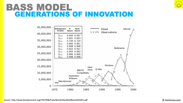
Again, it is interesting to see how close reality is to the mathematical curve.

For each generation, a familiar diffusion curve appears. Enough for us to be able to make predictions on production volumes, or service size, for innovations. Assuming we are accurate with our expected market size.

Additionally, we can see that the next incremental innovation was launching into the early adopters around the time the existing generation was drifting to the end of the late majority. This gives us an insight into the timing of innovation launching. Useful to keep in mind.

Do price and other attributes affect the model?

We don’t take account of price changes, advertising effort, or so on in the standard Bass Model. These variables can be called decision variables. And in Bass et al.’s paper “Why the Bass Model Fits without Decision Variables” a Generalised Bass Model is derived that takes account of decision variables.

I won’t go into that paper in this article. But, suffice to say, you can take account of decision variables in Bass’ model (the generalised version). And, if there are no decision variables to consider, then the generalised model reduces to the standard Bass Model.

You can find a more comprehensive discussion of the marketing mix influence on diffusion in the article “Modelling The Marketing-Mix Influence In New-Product Diffusion“.

Uses of diffusion models

We’ve seen a couple of applications of diffusion models above. In the book “New-product diffusion models” several more uses are identified in Table 1.1 on page 7. The article breaks down these use cases into two parts of the lifecycle: pre-launch & launch, and post-launch. And references are given to papers that back up the thinking.

Pre-launch & launch

As we have already seen, we can use diffusion models for product forecasting. What is the total number of sales expected? What and when is the expected peak. Therefore, we can model and understand supply chain needs. Minimising the risk of us overproducing and left with unsaleable stock.

We can also use the models to help with sampling. Which is the act of giving samples away to consumers in return for, hopefully, positive internal influencing. But how do we know how many samples to give, and to who to give them to? Diffusion models can help.

Post-launch

We have also already seen one post-launch use of diffusion models. When we touched on using them to model multi-generation innovations. We can use them to help identify the best timing to launch the next generation.

On the opposite end of oversupply is undersupply. We can use the diffusion model to help understand the waiting time if we undersupply the market. Or as the book puts it: “determination of the impact of capacity decisions on innovation diffusion”.

Two other, perhaps surprising, uses of diffusion models are to estimate pirated sales and losses of sales/market expansion due to patent infringements. Pirate sales, such as copying software, can be estimated by comparing actual sales to projections. And so can the impact of new entrant infringing patents. These need to be caveated with the model being correct. An incorrect model can incorrectly hint at pirating/infringement when it might just be your numbers were wrong.

We can even base the market valuation of a business on market penetration. Diffusion models give insight into what that penetration could be. And therefore help understand market valuations.

The final use suggested is as a tool for assessing market saturation and expansion opportunities for retailers.

Quite a useful tool, I hope you agree!

Wrapping Up

So, I think this is an advantageous model. And the set of papers referenced in this article are fascinating. But perhaps do not get the visibility deserved in the innovation community. For example, many can highlight Rogers’ 5 adopter types; fewer can draw the link to Bass’ model.

We have seen that under specific parameters, Bass’ model mimics Rogers adoption curve. Further, we saw that Bass’ model could be fit to a range of products sales data.

That also gives us the confidence to use the model as a prediction tool. And we saw that Bass did just that for colour TVs in the ’60s. Much to the anger of industry experts. His predictions were not far off; the industry’s predictions led to oversupply. Marketers have also used this approach to make predictions for “satellite television/telephone/radio, a new LCD projector, wireless telephones, and wireless Internet phones (3G)”.

To get predictions requires estimating the target market size and values for the coefficients p and q. Studies have given us average values and typical bounds on those coefficients. We can use these average values to check the relevance of our guesses.

Another useful empirical insight is the refinement of Rogers’ adopter type sizes from being standard deviations. We saw that innovators rather than being a standard, 2.5% are somewhere between 0.2 and 2.8%. Other adopter types similarly had ranges.

As a final note, Management Science’s 50th-anniversary edition noted Bass paper in the top 10 influential articles they had published.